The Dog That Didn't Bark Inside Your Language Model
Every production LLM satisfies a safety condition that had no name until this year. I found it by breaking it on purpose. Then I found a model that had bet everything on it.
There is a famous moment in Silver Blaze where Sherlock Holmes solves the case with a fact that did not happen. The dog did not bark in the night. Gregory, the Scotland Yard detective, protests that the dog did nothing. Holmes answers that this was the curious incident. A silence becomes evidence only against an expectation. Dogs bark at strangers. If there is no rule, there is no event. The dog that never barked at anyone tells you nothing. The dog that should have barked, and did not, tells you the intruder was familiar.
Every deployed language model satisfies a mathematical condition that, until this year, had no name. It had no name for exactly the reason the dog had no entry in Gregory’s notebook. The condition has never been violated. Not once, in any production model, by anyone. A condition that holds with probability 1 carries zero bits of surprise, and nobody names what never varies. So I did what Holmes did. I asked what should have been able to go wrong, and then I made it go wrong on purpose. Violating the condition inflates perplexity by up to 214x on production 7B models. A bit-identical control that preserves the condition changes nothing. Twenty-four cells out of twenty-four, at baseline.
One more thing before we start. The dog comes back at the end of this post. Not as a metaphor for how I found the condition, but as the literal shape of the mechanism, and then a third time, in a form I did not expect: a model where you can watch, layer by layer, which door each dog was trained to guard. Hold that thought.
1. The condition nobody named
Rotary Position Embedding (RoPE) is how most current LLMs know where a token is. It rotates 2D slices of the query and key vectors, and the k-th slice rotates with frequency
θ_k = b^(−2k/d), k = 0, 1, …, d/2 − 1.
That is the whole schedule. One base b (Llama-2 uses 10^4, Llama-3 uses 5x10^5, Mistral and Qwen2.5 use 10^6), one exponential, d/2 frequencies. In log space the frequencies form an arithmetic progression. Nothing else.
Now define a quantity nobody had defined: max_cluster, the size of the largest set of frequencies that share the same numerical value. Every deployed schedule has max_cluster = 1. All frequencies are pairwise distinct. Nobody designed this in. Nobody checks for it in any config file or test suite. It holds as a side effect of writing the schedule as an exponential, the way a spiral staircase never revisits a step.
Is this a real condition, or a tautology with a name? That is the right question to ask, because the schedule is full of exact numerical relations that do no harm at all. At b = 10^6 and d = 128, take k = 0 and k = 32. Then θ_0 = 1000 x θ_32, an exact rational ratio, sitting inside every Mistral checkpoint you have ever downloaded. The model does not care. So “the frequencies are related” cannot by itself be the dangerous thing. Something more specific is.
2. Breaking it on purpose
To find out whether max_cluster = 1 is load-bearing, you need an instrument that violates it while changing nothing else. Linear INT8 quantization of the frequency buffer turns out to be exactly that instrument. Quantization maps nearby values to the same bin. Apply symmetric linear INT8 to the d/2 = 64 frequencies of a b = 10^6 schedule and the smallest entries collapse together: 38 of the 64 channels land in a single bin. One rounding step, and max_cluster goes from 1 to 38.
I want to be precise about the role of quantization here, because it is easy to misread this as a paper about deployment bugs. Nobody’s production stack quantizes this buffer today. INT8 is the measuring device, not the threat model. It is a one-line, natural operation that manufactures a violation, the way Holmes manufactured his test by having Watson throw a smoke rocket. The threat model comes later, in Section 7.
So, the measurement. Two production models (Mistral-7B-v0.3 and Qwen2.5-7B), three datasets (WikiText-2, C4, PG-19), four context lengths from 2K to 16K. Perturb only the frequency buffer at inference time. Weights untouched.
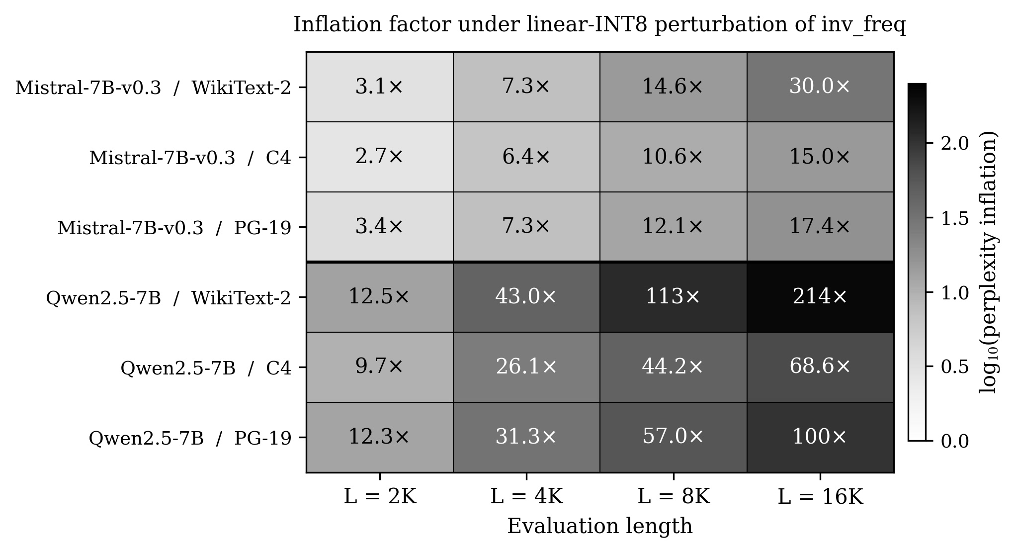
Every one of the 24 cells inflates. The factors run from 3.1x to 214x, and they grow monotonically with context length in every row. INT4, which produces even larger clusters, reaches 655x.
Here is the control, and the control is the whole point. Log-space INT8 quantization uses the identical bit budget and the identical arithmetic precision, but because the frequencies are a geometric sequence, quantizing in log space preserves their distinctness. max_cluster stays 1. Result: all 24 cells reproduce full-precision perplexity to within 0.1%. Same bits, same rounding, no clusters, no damage. Low-precision arithmetic is innocent. Cluster generation is the carrier.
3. The catastrophe is topological
Maybe the model is just sensitive to its frequency values, and any perturbation of this size would hurt? I tested that directly. Multiply every frequency by (1 + εξ) with random ξ, sweeping ε from 10^-5 up to 10^-2. That last one moves every single frequency by a full percent, far more numerical change than INT8 causes on most channels, but it keeps all values distinct. 240 cells, three seeds each.
Silence. Every cell within 0.1% of baseline. The attention pattern does not care where the frequencies are. It cares whether two of them are the same. Smooth motion inside the max_cluster = 1 stratum is invisible. Crossing the stratum boundary is a catastrophe. The failure is topological, not quantitative.
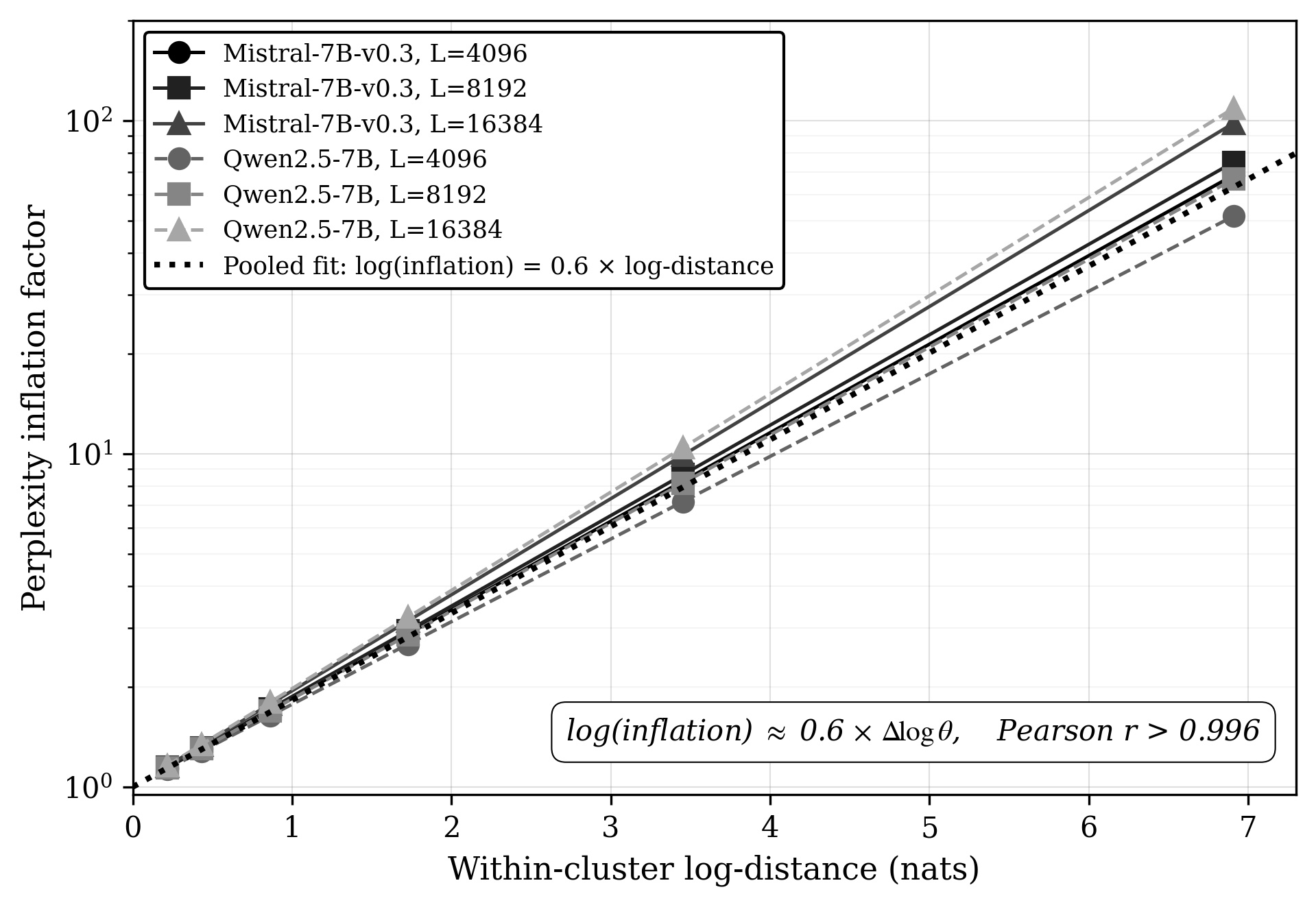
And once you are across the boundary, the damage is lawful. Fix the cluster size at 2 and vary the log-distance between the two merged frequencies. The inflation follows a clean power law:
log(inflation) ≈ 0.6 x Δlog θ, with Pearson r > 0.996,
and the slope is nearly the same across both models and all context lengths (fitted range 0.57 to 0.68). Doubling the log-distance multiplies the inflation by about 1.52. I did not expect a number this clean from a trained system, and I still find it a little eerie.
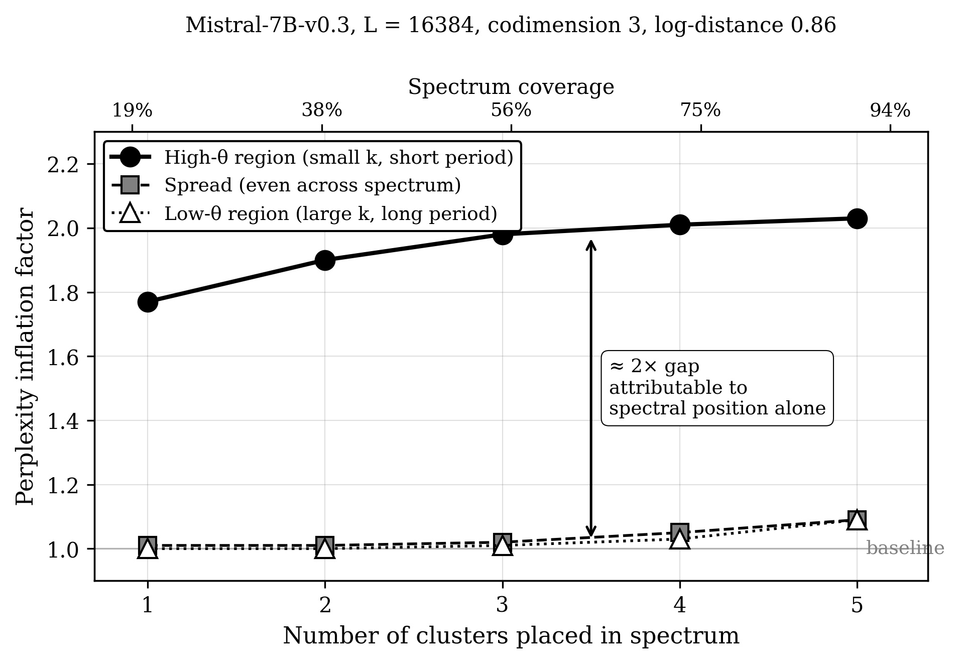
Where you place the cluster matters even more than how big it is. At fixed cluster size and fixed log-distance, a single small cluster at the high-frequency end of the spectrum inflates perplexity about 2x. Clusters at the low-frequency end stay near baseline even when they cover 94% of the spectrum. The high-frequency channels are where attention has trained hardest on fine position distinctions, and injected collisions there break what the training built.
4. Why you were safe all along
Now the question that made me write the paper instead of a notebook comment. The schedule already contains exact relations, like θ_0 = 1000 x θ_32. Injected clusters with far smaller log-distances are catastrophic. Why does trained attention tolerate the first and die from the second?
The answer needs one theorem from 1882. Every deployed base b is a positive rational other than 1, so by the Hermite-Lindemann theorem, log b is transcendental. Feed that through the schedule and you get two things. First, the frequencies are automatically pairwise distinct: max_cluster = 1 holds for free, for every deployed base, forever. Second, and this is the part the theorem really buys, the transcendence of log b pins down the schedule’s entire lattice of integer relations. The only relations that exist are the ones forced by the prime factorization of b. At b = 10^6 and d = 128, that means exactly the pairs (k, j) with 32 dividing k − j, generated by θ_0 = 1000 x θ_32, and nothing else. No accidental relations. The complete list is known.
So the training orbit of the model lives on a known sublattice, and attention grows its position-discriminating structure on that orbit. The relations the schedule carries were present during training. They are the household. A perturbation-induced cluster imposes a relation that was absent during training. The orbit collapses onto a sublattice the training distribution never covered, and at evaluation the model meets phase configurations it has no structure for.
Which is to say: the operative distinction is not large relation versus small relation. It is present-in-training versus injected-at-inference. Attention is the dog. It does not bark at θ_0 = 1000 x θ_32, not because that relation is far away, but because that relation is familiar. It grew up in the house. It barks catastrophically at an injected cluster of equal or smaller log-distance, because that one is a stranger. (There is a reading of the Holmes scene, due to Žižek, that says an absence becomes an event only inside a symbolic order that expected a presence. I mention it because the mechanism here is that reading, executed in float16.)
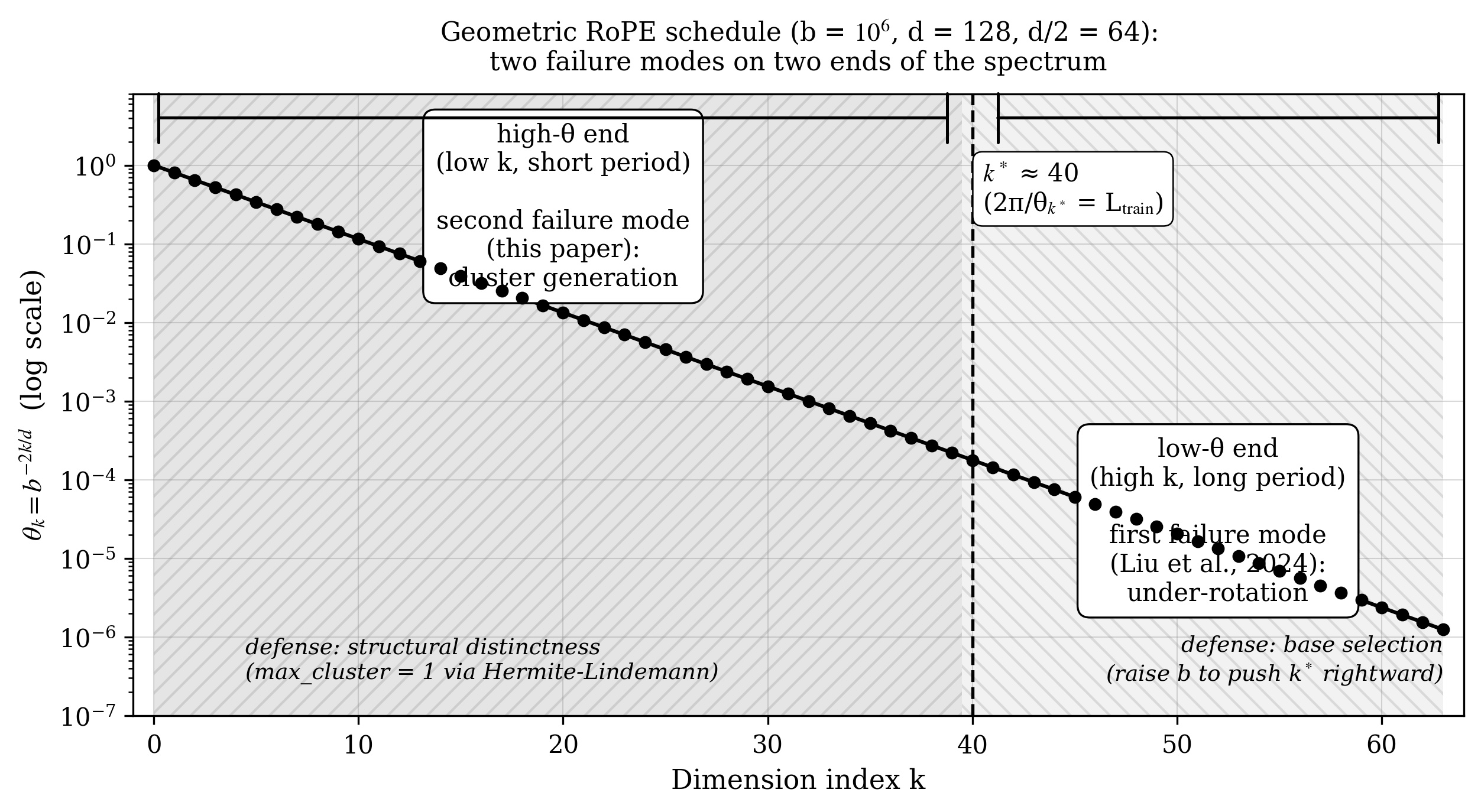
The two known failure modes of RoPE now sit in one picture. Liu et al. (ICLR 2024) showed that the low-frequency end fails by under-rotation when you extrapolate past the training length, and the cure is base selection. The failure mode above lives at the high-frequency end and is guarded by structural distinctness, which the geometric form provides for free via transcendence. Two ends of the spectrum, two independent defenses, both accidental gifts of writing the schedule as one exponential.
If the post ended here, the story would be static. A hidden condition, a free theorem, everyone safe. Then I opened a hybrid model, and the story acquired a second act that partially inverts the first.
5. Same intruder, different dogs
Gemma-3-4B interleaves two kinds of attention layers. Sliding-window layers see a local window of 1024 tokens and use RoPE base 1e4. Full-attention layers see everything and use base 1e6 stretched by a factor 8 position interpolation. DeepMind’s technical report shows this design works. It does not ask how the two layer types differ under the hood, and that turned out to be where the interesting thing lives.
I ran the same codimension-2 cluster injection on each layer type separately. Same arithmetic, same injection, same model.
The sliding layers fail catastrophically, up to 198x at the worst configuration. The full-attention layers are immune. Not resistant. Immune, at baseline, under the same injection that multiplies the sliding layers’ perplexity by two hundred.
Ablation tells you why. Zero out the low-frequency channels of the full-attention layers and nothing happens, which means those layers do not use their low frequencies for position at all. Zero out their high-frequency channels and you get 1.04x, a shrug. The full layer holds its positional information loosely, spread out, redundant. The sliding layer holds its frequencies tightly and cannot afford to lose distinctness anywhere.
This is the third dog, and it completes the equation from Section 4. Vulnerability equals trained reliance. The full-attention layer is a dog that never guarded that particular door, so an intruder there gets silence, not because the dog is calm but because that entrance was never its post. The sliding layer guards that door with everything it has. Same intruder, different training, opposite outcome. And note what this does to the mechanism question: the two layer types share the same frequency arithmetic, so arithmetic cannot explain the asymmetry. The remaining variable is what each layer learned to depend on. I also tested the geometric alternative directly (conditioning of the feature matrix) and it moves monotonically in base, which fails to match the data. Elimination on one side, the layer asymmetry as positive evidence on the other.
6. The best-looking point is the all-in point
Here is the measurement I keep coming back to. Take the sliding layers and sweep the RoPE base across six values from 3e3 to 1e6, measuring baseline perplexity at each. The curve is a U. Its minimum sits at 1e4. That is the value DeepMind shipped, so their tuning found the perplexity optimum, which is what good tuning does.
Now inject the same codimension-2 cluster at each base and measure the inflation. At base 3e4, one step from the optimum, the injection costs 1.43x, and baseline perplexity is nearly unchanged (6.98 against 6.65). At base 1e4, the optimum itself, the same injection costs 197x.
Read that pair of numbers slowly. The point that looks best on the metric is the point where the model has bet everything on frequency distinctness. This is not a coincidence of two unrelated curves, or at least the layer evidence says it is not. A base of 1e4 inside a 1024-token window gives the layer a frequency set it can use tightly, every channel earning its place in position discrimination. That tight use is exactly what the perplexity optimum rewards, and exactly what leaves no redundancy to absorb a loss of distinctness. The same training pressure that pushes the metric down concentrates the reliance. One step away, at 3e4, the layer uses its frequencies more loosely, pays 5% perplexity for it, and shrugs off the injection that destroys the optimum.
To a LessWrong reader this rhymes with a familiar pattern: optimize the visible metric and you may be purchasing invisible fragility, because the metric does not price robustness. I want to state clearly how far the data licenses that reading and where it stops. What is measured: the optimum and the fragility peak coincide in this model, the coincidence survives a direct test of the geometric alternative, and the layer asymmetry positively locates the mechanism in trained reliance rather than frequency arithmetic. What is not established: this is one model, the base sweep swaps the base at inference time so a training mismatch is mixed into every off-optimum point, the 1e6 endpoint of the sweep is contaminated by that mismatch, and the mechanism behind the coincidence of the two extrema is open. If someone retrains the sliding layers at 3e4 and the robustness gap survives, this becomes a design result. Until then it is a measured tension, and I would rather under-claim it than decorate it.
7. What quantization actually does to the tight dog
Section 2 used INT8 as an instrument. On Gemma’s sliding layers it stops being hypothetical in an instructive way. Apply linear INT8 to the sliding-layer frequency buffer and 42 channels merge (log-space INT8: zero merges). Perplexity inflates 24.95x (log-space: 1.00x). The linear-versus-log split replicates on a third production model, in a different base family, inside a hybrid architecture.
But the useful part is where the damage lands. Decompose the loss by position:
positions 0 to 16: Δloss +0.003 positions 16 to 64: +0.060 positions 64 to 256: +0.040 positions 256 to 512: +0.004 positions 512 to 1024: +1.303
The model is fine at short range and collapses specifically at long range, right at the window boundary. That pattern has a clean mechanical reading. In the buffer as HuggingFace stores it, the small entries are the low frequencies, the long-wavelength channels that discriminate distant positions, and linear quantization’s zero bin swallows precisely those. (You can check the direction yourself in three lines: build inv_freq for b = 1e6, d = 128, quantize, and look at which k merge. It is the tail, k = 26 to 63, thirty-eight channels into one bin at value zero.) Short-range discrimination lives in the surviving high-frequency channels, so short context looks healthy and the failure hides until the context grows. Which also retro-explains the cleanest regularity of Section 2: inflation grows monotonically with evaluation length in every single row, because what the cluster destroyed was long-range discrimination all along.
So the practical sentence, for anyone who ships quantized long-context models: if you ever quantize a RoPE frequency buffer, quantize in log space. Same bits, no clusters, no damage. It is the cheapest mitigation I have ever measured.
8. Who should start checking
The geometric form protects you for free, so as long as everyone uses it, max_cluster = 1 is a curiosity. Three current directions stop using it, and they are exactly the readers I hope reach this section.
Learned per-dimension schedules (LongRoPE and its family) replace the exponential with searched or trained scales. The parameterization no longer guarantees distinctness, and a search optimizing only long-context perplexity has no term telling it not to land two scaled frequencies on the same value. The condition should be a constraint or a regularizer there, and it costs one line.
Frequency-merging compression is already here. Recent KV-cache and GQA-to-MLA work folds nearby RoPE frequencies on purpose and observes, empirically, that some layers tolerate large folds while middle layers need exact frequencies. From where this post stands, those groups are rediscovering the map of Section 5 by hand: fold tolerance is trained reliance, layer by layer. The distinction that predicts safety is whether the merged relation was present in training or is being injected after it, and that is checkable from the schedule and the checkpoint before you deploy anything.
Low-precision inference below eight bits, including fp8 pipelines, moves rounding ever closer to the frequency buffer. The zero-bin mechanism of Section 7 is one cast operation away, and it hides at short context by construction.
The condition is one integer to compute. max_cluster of your frequency tuple, after every transformation your pipeline applies to it. If it is 1, your dog is asleep because the house is quiet. If it is not, Section 2 is a preview of your perplexity, and the short-context evals you ran will not have warned you.
The full measurements and the transcendence argument are in the paper, “Twos All the Way Down: A Hidden Condition Every Deployed RoPE Schedule Satisfies” (Zenodo, DOI 10.5281/zenodo.20510387), currently under review at the Machine Learning journal (ACML 2026 track). The Gemma-3 measurements in Sections 5 to 7 are from follow-up work in preparation. Code for every table and figure is available on request and will be public with the revision. If you spot an error, I would genuinely rather hear it now than in August.
How to cite
For the condition, the 24-cell survey, the power law, and the transcendence argument (Sections 1 to 4), cite the paper:
@misc{ryu2026twos,
  author = {Ryu, Sungmin},
  title  = {Twos All the Way Down: A Hidden Condition Every Deployed RoPE Schedule Satisfies},
  year   = {2026},
  doi    = {10.5281/zenodo.20510387},
  note   = {Under review, Machine Learning (ACML 2026 journal track)}
}
The Gemma-3 hybrid measurements and the base-sweep result (Sections 5 to 7) are not yet in any paper. Until the follow-up manuscript is out, this post is the primary source:
@misc{ryu2026dog,
  author = {Ryu, Sungmin},
  title  = {The Dog That Didn't Bark Inside Your Language Model},
  year   = {2026},
  url    = {https://USERNAME.github.io/2026/07/14/dog-that-didnt-bark.html},
  note   = {Blog post}
}